Post-Secondary Employment Outcomes (PSEO)
Post-Secondary Employment Outcomes (PSEO) are experimental tabulations developed by researchers at the U.S. Census Bureau. PSEO data provide earnings and employment outcomes for college and university graduates by degree level, degree major, post-secondary institution, and state of institution. These statistics are generated by matching university transcript data with a national database of jobs, using state-of-the-art confidentiality protection mechanisms to protect the underlying data. The PSEO are made possible through data sharing partnerships between universities, university systems, State Departments of Education, State Labor Market Information offices, and the U.S. Census Bureau. PSEO data are available for post-secondary institutions whose transcript data have been made available to the Census Bureau through a data-sharing agreement.
Since this documentation is focused on code samples, it will not detail all the specifics of the PSEO data. For more information, users may find the following links/resources useful:
PSEO Explorer: PSEO Explorer is an interactive tool that allows for comparisons of employment outcomes through dynamic grouped bar charts and employment flows through Sankey diagrams.
PSEO Information and Coverage: This webpage provides background and information about which states and universities/university systems contribute to the data.
PSEO Help and Documentation: This webpage provides background information on PSEO methodology and other useful topics.
PSEO Technical Documentation: This document provides information on the construction of the PSEO data as well as information on the disclosure status of the PSEO data product and Census Bureau Disclosure Review Board approval numbers.
PSEO Schema for Latest Release: This schema provides detailed information on file naming, structure, identifiers, and indicators.
PSEO Files in a Directory Structure: The code samples in this documentation utilize the files from this URL.
Reading Data Files
PSEO data can be accessed in two ways, either through the Census API or directly from the online directory structure. Either can be used to conduct analyses, as the data is the same, but users may have a preference for one method or the other depending on preference or project requirements. Below both methods are detailed, but the remaining PSEO code samples will use the data files directly.
Using the Online Directory Structure
Here, the files are read directly from the online directory structure, but the same code can be used for reading the files locally instead. When selecting PSEO files to read/download, there are two main considerations:
Earnings or Flows: PSEO Earnings data provides access to earnings at the 25th, 50th, and 75th percentile at 1, 5, and 10 years post graduation. Flows provide counts of employed graduates by industry and geography, 1, 5, and 10 years after graduation. These files have separate structures, but can be merged at several levels, if needed.
State or All: PSEO earnings and flows data can be downloaded for a specific state, or for “all”. If downloaded for a specific state, the file will contain information on graduates from institutions in that state only. The “all” files contain all data for earnings or flows (essentially, all the individual state files stacked on top of each other).
In the example below, the earnings file for Colorado is read directly from the online directory structure. This file contains earnings data for all institutions in Colorado. After reading in the data, this code limits the file to the highest level aggregation. In this case, that is earnings from all PSEO-participating institutions in Colorado, across all CIP codes (for more on CIP codes, see the National Center for Education Statistics and/or the LEHD Schema), and across all graduation cohorts. Degree level is also present as we do not aggregate across degree levels. Therefore, the earnings numbers below can be interpreted as the median earnings 1 year after graduation by degree level for graduates from institutions in Colorado across all instructional programs (CIP codes) and all cohorts. The results also include the number of graduates we observe with sufficient labor force attachment. (i.e. the number of graduates used to calculate the earnings figures) as well as a status flag. Information on the coding of degree_types can be found in the LEHD Schema, and for an example of joining schema labels to data, see Case Study: How Many Engineering Graduates Stay in Illinois?.
Note
The structure of the PSEO data may not be immediately intuitive to data users. For example, in the code below, the institution of 08 corresponds to “All Institutions in Colorado”. The most helpful resource for understanding the structure of PSEO data is the LEHD Schema. Some potentially helpful places to start are Identifiers for PSEO, Indicators for PSEO Earnings, and Indicators for PSEO Flows.
import pandas as pd

STATE = "co"
BASE_URL = "https://lehd.ces.census.gov/data/pseo/latest_release/"


# Read Colorado earnings CSV (gzipped)
colorado_earnings = pd.read_csv(
    f"{BASE_URL}{STATE}/pseoe_{STATE}.csv.gz",
    dtype={"institution": str, "degree_level": str, "cipcode": str, "grad_cohort": str},
    low_memory=False,
)

# Display 50th percentile earnings for all Colorado Grads for all CIP Codes
# and all graduation cohorts by degree type
all_colorado_grads = colorado_earnings.loc[
    (colorado_earnings["institution"] == "08")
    & (colorado_earnings["cipcode"] == "00")
    & (colorado_earnings["grad_cohort"] == "0000"),
    ["y1_p50_earnings", "degree_level", "y1_grads_earn", "status_y1_earnings"],
]

print(all_colorado_grads)
>> y1_p50_earnings degree_level y1_grads_earn status_y1_earnings >> 0 34540.0 01 78464.0 1 >> 1 40177.0 02 26145.0 1 >> 2 37982.0 03 79020.0 1 >> 3 NaN 04 NaN 5 >> 4 40501.0 05 305134.0 1 >> 5 47119.0 06 62.0 1 >> 6 62915.0 07 88900.0 1 >> 7 NaN 08 NaN 5 >> 8 72856.0 17 10500.0 1 >> 9 75701.0 18 10524.0 1
library(readr)
library(dplyr)

state <- "co"
base_url <- "https://lehd.ces.census.gov/data/pseo/latest_release/"

# Read Colorado earnings CSV (gzipped)
colorado_earnings <- read_csv(
  paste0(base_url, state, "/pseoe_", state, ".csv.gz"),
  col_types = cols(
    institution = col_character(),
    degree_level = col_character(),
    cipcode = col_character(),
    grad_cohort = col_character()
  )
)

# Display 50th percentile earnings for all Colorado Grads for all CIP Codes
# and all graduation cohorts by degree type
all_colorado_grads <- colorado_earnings %>%
  filter(
    institution == "08",
    cipcode == "00",
    grad_cohort == "0000"
  ) %>%
  select(y1_p50_earnings, degree_level, y1_grads_earn, status_y1_earnings)

print(all_colorado_grads)
>> # A tibble: 10 × 4 >> y1_p50_earnings degree_level y1_grads_earn status_y1_earnings >> <dbl> <chr> <dbl> <dbl> >> 1 34540 01 78464 1 >> 2 40177 02 26145 1 >> 3 37982 03 79020 1 >> 4 NA 04 NA 5 >> 5 40501 05 305134 1 >> 6 47119 06 62 1 >> 7 62915 07 88900 1 >> 8 NA 08 NA 5 >> 9 72856 17 10500 1 >> 10 75701 18 10524 1
A very similar method can be used to read the flows data. Here, the Colorado flows data is read, and then is limited to a subset. In the flows data, there is essentially a cross between which industry a graduate is employed in and which geographic region they are employed in. The data displayed below is thus the number of graduates from Masters programs in Colorado who are employed in each Census division 1 year after graduation. Here, the code selects data for “All NAICS Sectors”, but we could also cross geography with industry (i.e. for a specific NAICS sector, how many graduates are employed in each Census division). It’s worth noting the two other columns in the data in addition to y1_grads_emp. First, y1_grads_emp_instate details the number of graduates who are employed in the same state as the degree is from (in this case Colorado). This column will only contain a non-zero number for the national geography flow and for the Census division that contains the institution state (Colorado is in Census division 8). Second, y1_grads_nme indicates the number of graduates who have no (or only marginal) earnings in the LEHD data. This number will only be reported for the national geography flow.
import pandas as pd

STATE = "co"
BASE_URL = "https://lehd.ces.census.gov/data/pseo/latest_release/"


# Read Colorado earnings CSV (gzipped)
colorado_flows = pd.read_csv(
    f"{BASE_URL}{STATE}/pseof_{STATE}.csv.gz",
    dtype={
        "institution": str,
        "degree_level": str,
        "cipcode": str,
        "grad_cohort": str,
        "geography": str,
    },
    low_memory=False,
)

# Limit to Geographic flows for all masters students in Colorado
colorado_flows_limited = colorado_flows[
    (colorado_flows["institution"] == "08")
    & (colorado_flows["grad_cohort"] == "0000")
    & (colorado_flows["degree_level"] == "07")
    & (colorado_flows["cipcode"] == "00")
    & (colorado_flows["industry"] == "00")
]

# View Y1 grad counts by geography
print(
    colorado_flows_limited[
        ["geography", "y1_grads_emp", "y1_grads_emp_instate", "y1_grads_nme"]
    ]
)
>> geography y1_grads_emp y1_grads_emp_instate y1_grads_nme >> 6 00 96065.0 67693.0 37376.0 >> 155769 1 735.0 0.0 NaN >> 155770 2 2332.0 0.0 NaN >> 155771 3 3442.0 0.0 NaN >> 155772 4 2408.0 0.0 NaN >> 155773 5 4590.0 0.0 NaN >> 155774 6 786.0 0.0 NaN >> 155775 7 3619.0 0.0 NaN >> 155776 8 71319.0 67693.0 NaN >> 155777 9 6834.0 0.0 NaN
library(readr)
library(dplyr)

state <- "co"
base_url <- "https://lehd.ces.census.gov/data/pseo/latest_release/"

# Read Colorado earnings CSV (gzipped)
colorado_flows <- read_csv(
  paste0(base_url, state, "/pseof_", state, ".csv.gz"),
  col_types = cols(
    institution = col_character(),
    degree_level = col_character(),
    cipcode = col_character(),
    grad_cohort = col_character(),
    geography = col_character()
  )
)

# Limit to Geographic flows for all masters students in Colorado
colorado_flows_limited <- colorado_flows %>%
  filter(
    institution == "08",
    grad_cohort == "0000",
    degree_level == "07",
    cipcode == "00",
    industry == "00"
  )

# View Y1 grad counts by geography
print(colorado_flows_limited %>%
  select(geography, y1_grads_emp, y1_grads_emp_instate, y1_grads_nme))
>> # A tibble: 10 × 4 >> geography y1_grads_emp y1_grads_emp_instate y1_grads_nme >> <chr> <dbl> <dbl> <dbl> >> 1 00 96065 67693 37376 >> 2 1 735 0 NA >> 3 2 2332 0 NA >> 4 3 3442 0 NA >> 5 4 2408 0 NA >> 6 5 4590 0 NA >> 7 6 786 0 NA >> 8 7 3619 0 NA >> 9 8 71319 67693 NA >> 10 9 6834 0 NA
Using the Census API
To use the Census API, first the user should request an API key. Note that limited queries can be made without an API key (simply leave off the &key= portion of the request), but that for repeated queries, an API key should be used. Documentation on the PSEO API is available here. The API has two endpoints, one for flows and one for earnings. To use the API, a user should be very familiar with the PSEO data structure. This code produces the same data/output as that in Using the Online Directory Structure, but behaves slightly differently. Instead of reading all of the Colorado data from the API, the code tailors the request to the API to produce only the data needed. If a user has a very specific data need or has memory constraints, the API may therefore be a better choice.
import pandas as pd
import requests

# Define your API Key (Get one from https://api.census.gov/data/key_signup.html)
API_KEY = "YOUR_API_KEY_HERE"
if API_KEY == "YOUR_API_KEY_HERE":
    raise ValueError("Please create and enter your own API Key before continuing.")

# Define the base URL for PSEO Earnings
BASE_URL = "https://api.census.gov/data/timeseries/pseo/earnings"

# Define the indicators desired (50 percentile earnings 1 year post graduation, number of grads, and status)
INDICATORS = [
    "Y1_P50_EARNINGS",
    "Y1_GRADS_EARN",
    "STATUS_Y1_EARNINGS",
]

# Want to see results by degree_level
IDENTIFIERS = ["DEGREE_LEVEL"]

# Pick variables
# State level data for all grad cohorts and all cip CODES
STATE = "08"
GRAD_COHORT = "0000"
CIP_CODE = "00"

# Construct the API request URL
url = f"{BASE_URL}?get={','.join(INDICATORS + IDENTIFIERS)}&for=us:1&INSTITUTION={STATE}&GRAD_COHORT={GRAD_COHORT}&CIPCODE={CIP_CODE}&key={API_KEY}"

# Make the request
response = requests.get(url)
data = response.json()

# Convert to DataFrame
pseo_earnings = pd.DataFrame(data[1:], columns=data[0])

# Display 50th percentile earnings for all Colorado Grads for all CIP Codes
# and all graduation cohorts by degree type
print(
    pseo_earnings[
        ["Y1_P50_EARNINGS", "DEGREE_LEVEL", "Y1_GRADS_EARN", "STATUS_Y1_EARNINGS"]
    ]
)
>> Y1_P50_EARNINGS DEGREE_LEVEL Y1_GRADS_EARN STATUS_Y1_EARNINGS >> 0 34540 01 78464 1 >> 1 40177 02 26145 1 >> 2 37982 03 79020 1 >> 3 None 04 None 5 >> 4 40501 05 305134 1 >> 5 47119 06 62 1 >> 6 62915 07 88900 1 >> 7 None 08 None 5 >> 8 72856 17 10500 1 >> 9 75701 18 10524 1
library(httr)
library(jsonlite)
library(dplyr)

# API key
api_key <- "YOUR_API_KEY_HERE"
if (api_key == "YOUR_API_KEY_HERE") {
  stop("Please create and enter your own API Key before continuing.")
}

# Base URL and query parameters
base_url <- "https://api.census.gov/data/timeseries/pseo/earnings"

# Define the indicators desired (50 percentile earnings 1 year post graduation, number of grads, and status)
indicators <- c("Y1_P50_EARNINGS", "Y1_GRADS_EARN", "STATUS_Y1_EARNINGS")

# Want to see results by degree_level
identifiers <- c("DEGREE_LEVEL")

# Pick variables
# State level data for all grad cohorts and all cip CODES
state <- "08"
grad_cohort <- "0000"
cip_code <- "00"

# Construct the API request URL
query_url <- paste0(
  base_url,
  "?get=", paste(c(indicators, identifiers), collapse = ","),
  "&for=us:1",
  "&INSTITUTION=", state,
  "&GRAD_COHORT=", grad_cohort,
  "&CIPCODE=", cip_code,
  "&key=", api_key
)

# Make the request
response <- GET(query_url)
json_data <- content(response, "text")
parsed_data <- fromJSON(json_data)

# Convert to data frame
colnames(parsed_data) <- parsed_data[1, ]
pseo_earnings <- as.data.frame(parsed_data[-1, ])


# Display 50th percentile earnings for all Colorado Grads for all CIP Codes
# and all graduation cohorts by degree type
pseo_earnings <- pseo_earnings %>% select(Y1_P50_EARNINGS, DEGREE_LEVEL, Y1_GRADS_EARN, STATUS_Y1_EARNINGS)
print(pseo_earnings)
>> Y1_P50_EARNINGS DEGREE_LEVEL Y1_GRADS_EARN STATUS_Y1_EARNINGS >> 1 34540 01 78464 1 >> 2 40177 02 26145 1 >> 3 37982 03 79020 1 >> 4 <NA> 04 <NA> 5 >> 5 40501 05 305134 1 >> 6 47119 06 62 1 >> 7 62915 07 88900 1 >> 8 <NA> 08 <NA> 5 >> 9 72856 17 10500 1 >> 10 75701 18 10524 1
The flows code from Using the Online Directory Structure is likewise replicated below with the API. Again, just the specific desired data is requested from the API. One difference to note here is that the call below does not produce a total (national) row. To get this row (and the number of graduates “not meaningfully employed”), the “for” statement (i.e. for=division:*) needs to be modified to be for=us:1 to receive national data.
import pandas as pd
import requests

# Define your API Key (Get one from https://api.census.gov/data/key_signup.html)
API_KEY = "YOUR_API_KEY_HERE"
if API_KEY == "YOUR_API_KEY_HERE":
    raise ValueError("Please create and enter your own API Key before continuing.")

# Define the base URL for PSEO Flows
BASE_URL = "https://api.census.gov/data/timeseries/pseo/flows"

# Define the indicators desired (grads employed 1 year after graduation)
INDICATORS = ["Y1_GRADS_EMP", "Y1_GRADS_EMP_INSTATE", "Y1_GRADS_NME"]

# Want to see results by division
IDENTIFIERS = [
    "DIVISION",
]

# Pick variables
# State level data for all grad cohorts and all cip CODES
# All industries
STATE = "08"
GRAD_COHORT = "0000"
DEGREE_LEVEL = "07"
CIPCODE = "00"
NAICS = "00"

# Construct the API request URL
url = f"{BASE_URL}?get={','.join(INDICATORS + IDENTIFIERS)}&for=division:*&INSTITUTION={STATE}&GRAD_COHORT={GRAD_COHORT}&DEGREE_LEVEL={DEGREE_LEVEL}&CIPCODE={CIPCODE}&NAICS={NAICS}&key={API_KEY}"

# Make the request
response = requests.get(url)
data = response.json()

# Convert to DataFrame
pseo_flows = pd.DataFrame(data[1:], columns=data[0])

# View Y1 grad counts by geography
print(pseo_flows[["DIVISION", "Y1_GRADS_EMP", "Y1_GRADS_EMP_INSTATE", "Y1_GRADS_NME"]])
>> DIVISION Y1_GRADS_EMP Y1_GRADS_EMP_INSTATE Y1_GRADS_NME >> 0 1 735 0 None >> 1 2 2332 0 None >> 2 3 3442 0 None >> 3 4 2408 0 None >> 4 7 3619 0 None >> 5 8 71319 67693 None >> 6 9 6834 0 None >> 7 5 4590 0 None >> 8 6 786 0 None
library(httr)
library(jsonlite)
library(dplyr)

# Define your API Key (Get one from https://api.census.gov/data/key_signup.html)
api_key <- "YOUR_API_KEY_HERE"
if (api_key == "YOUR_API_KEY_HERE") {
  stop("Please create and enter your own API Key before continuing.")
}

# Define the base URL for PSEO Flows
base_url <- "https://api.census.gov/data/timeseries/pseo/flows"

# Define the indicators desired (grads employed 1 year after graduation)
indicators <- c("Y1_GRADS_EMP", "Y1_GRADS_EMP_INSTATE", "Y1_GRADS_NME")

# Want to see results by division
identifiers <- c("DIVISION")

# Pick variables
# State level data for all grad cohorts and all cip CODES
# All industries
state <- "08"
grad_cohort <- "0000"
degree_level <- "07"
cip_code <- "00"
naics <- "00"

# Construct the API request URL
query_url <- paste0(
  base_url,
  "?get=",
  paste(c(indicators, identifiers), collapse = ","),
  "&for=division:*",
  "&INSTITUTION=", state,
  "&GRAD_COHORT=", grad_cohort,
  "&DEGREE_LEVEL=", degree_level,
  "&CIPCODE=", cip_code,
  "&NAICS=", naics,
  "&key=", api_key
)

# Make the request
response <- GET(query_url)
json_data <- content(response, "text")
parsed_data <- fromJSON(json_data)

# Convert to data frame
colnames(parsed_data) <- parsed_data[1, ]
pseo_flows <- as.data.frame(parsed_data[-1, ])

# View Y1 grad counts by geography
print(pseo_flows %>%
  select(DIVISION, Y1_GRADS_EMP, Y1_GRADS_EMP_INSTATE, Y1_GRADS_NME))
>> DIVISION Y1_GRADS_EMP Y1_GRADS_EMP_INSTATE Y1_GRADS_NME >> 1 1 735 0 <NA> >> 2 2 2332 0 <NA> >> 3 3 3442 0 <NA> >> 4 4 2408 0 <NA> >> 5 7 3619 0 <NA> >> 6 8 71319 67693 <NA> >> 7 9 6834 0 <NA> >> 8 5 4590 0 <NA> >> 9 6 786 0 <NA>
Visualizing Data Over Time
In some cases, PSEO earnings data may cover cohorts across 20 years. Currently, PSEO Explorer does not support easy visualization over time, so users may wish to do this on their own.
Case Study: Earnings over Time for Graduates in Engineering
The code below visualizes earnings over time for bachelor’s degree earners in Illinois. Specifically, let’s analyze median earnings at 1, 5, and 10 years. Luckily, all earnings data in PSEO is converted to current dollars, so the comparison is valid. The first step is to retrieve the data (all earnings data for Illinois), and then subset to just the data we are interested in. Filtering the data is based on the values from the schema: for example the degree_level of “05” corresponds to “Baccalaureate”. A user may want to join these labels to the data, especially in the case of industry or institution name. For an example of this, see the example in Case Study: How Many Engineering Graduates Stay in Illinois?
Then, we can examine the “status” variables. These variables indicate the status of the data (for more information, see the LEHD Schema), with 1 indicating an “OK” status. As is visible in the output below, there are several rows in which there are status flags with a value of “-1”, indicating “data not available to compute this estimate”. This is because the data is not yet available for 5 and 10 years out of the most recent cohorts.
import pandas as pd
import matplotlib.pyplot as plt

STATE = "il"
BASE_URL = "https://lehd.ces.census.gov/data/pseo/latest_release/"

# Read in illinois earnings CSV (gzipped)
il_earnings = pd.read_csv(
    f"{BASE_URL}{STATE}/pseoe_{STATE}.csv.gz",
    dtype={
        "institution": str,
        "degree_level": str,
        "cipcode": str,
        "cip_level": str,
        "grad_cohort": str,
    },
)

# Filter to state-level earnings, bachelor's degrees, and engineers only
il_earnings = il_earnings[il_earnings["institution"] == "17"]
il_earnings = il_earnings[il_earnings["degree_level"] == "05"]
il_earnings = il_earnings[il_earnings["cipcode"] == "14"]

# Remove all years cohort
il_earnings = il_earnings[il_earnings["grad_cohort"] != "0000"]

# Filter rows where any of the three status variables are not 1
rows_with_bad_status = il_earnings[
    (il_earnings["status_y1_earnings"] != 1)
    | (il_earnings["status_y5_earnings"] != 1)
    | (il_earnings["status_y10_earnings"] != 1)
]

print(
    rows_with_bad_status[
        [
            "grad_cohort",
            "status_y1_earnings",
            "status_y5_earnings",
            "status_y10_earnings",
        ]
    ]
)
>> grad_cohort status_y1_earnings status_y5_earnings status_y10_earnings >> 1738 2013 1 1 -1 >> 1812 2016 1 -1 -1 >> 1958 2019 1 -1 -1
library(readr)
library(dplyr)
library(ggplot2)
library(tidyr)

STATE <- "il"
BASE_URL <- "https://lehd.ces.census.gov/data/pseo/latest_release/"

# Read in Illinois earnings CSV (gzipped)
il_earnings <- read_csv(
  paste0(BASE_URL, STATE, "/pseoe_", STATE, ".csv.gz"),
  col_types = cols(
    institution = col_character(),
    degree_level = col_character(),
    cip_level = col_character(),
    cipcode = col_character(),
    grad_cohort = col_character()
  )
)

# Filter to state-level earnings, bachelor's degrees, and engineers only
il_earnings <- il_earnings %>%
  filter(
    institution == "17", # State-level data
    degree_level == "05", # Bachelor's degrees
    cipcode == "14", # Engineering CIP code
    grad_cohort != "0000" # Remove all-years cohort
  )

# Ensure grad_cohort is sorted
df <- il_earnings %>% arrange(grad_cohort)

# Filter rows where any of the three status variables are not 1
rows_with_bad_status <- il_earnings[
  il_earnings$status_y1_earnings != 1 |
    il_earnings$status_y5_earnings != 1 |
    il_earnings$status_y10_earnings != 1,
]

print(rows_with_bad_status[, c("grad_cohort", "status_y1_earnings", "status_y5_earnings", "status_y10_earnings")])
>> # A tibble: 3 × 4 >> grad_cohort status_y1_earnings status_y5_earnings status_y10_earnings >> <chr> <dbl> <dbl> <dbl> >> 1 2013 1 1 -1 >> 2 2016 1 -1 -1 >> 3 2019 1 -1 -1
Since the status of the data is acceptable, we can plot the data. For bachelor’s degrees, the cohort length is three years, and the year in the data file is the start year of the cohort. Therefore, the graph produced by the code below represents the median earnings at 1, 5, and 10 years after graduation for each 3-year cohort.
Warning
When analyzing PSEO data at any level of data, it is important to be careful of composition effects. This is especially true at the state level. The institutions available in the PSEO data may not be a representative sample of all institutions in a given state, and should not be construed as such. Institutions may add new programs over time, so a trend over time could be a result of more/different graduates, rather than a true trend. It’s also possible for institutions to enter and leave the data in the middle of a time series.
# Ensure grad_cohort is sorted
il_flows = il_earnings.sort_values("grad_cohort")
# Plotting by year over time
plt.figure(figsize=(10, 6))

plt.plot(
    il_flows["grad_cohort"], il_flows["y1_p50_earnings"], marker="o", label="1 Year"
)
plt.plot(
    il_flows["grad_cohort"], il_flows["y5_p50_earnings"], marker="s", label="5 Years"
)
plt.plot(
    il_flows["grad_cohort"], il_flows["y10_p50_earnings"], marker="^", label="10 Years"
)

plt.title("Median Earnings of Illinois Engineering Bachelor Graduates by Cohort")
plt.xlabel("Graduation Cohort")
plt.ylabel("Median Earnings (2022 Dollars)")
plt.legend()
plt.grid(True)
plt.tight_layout()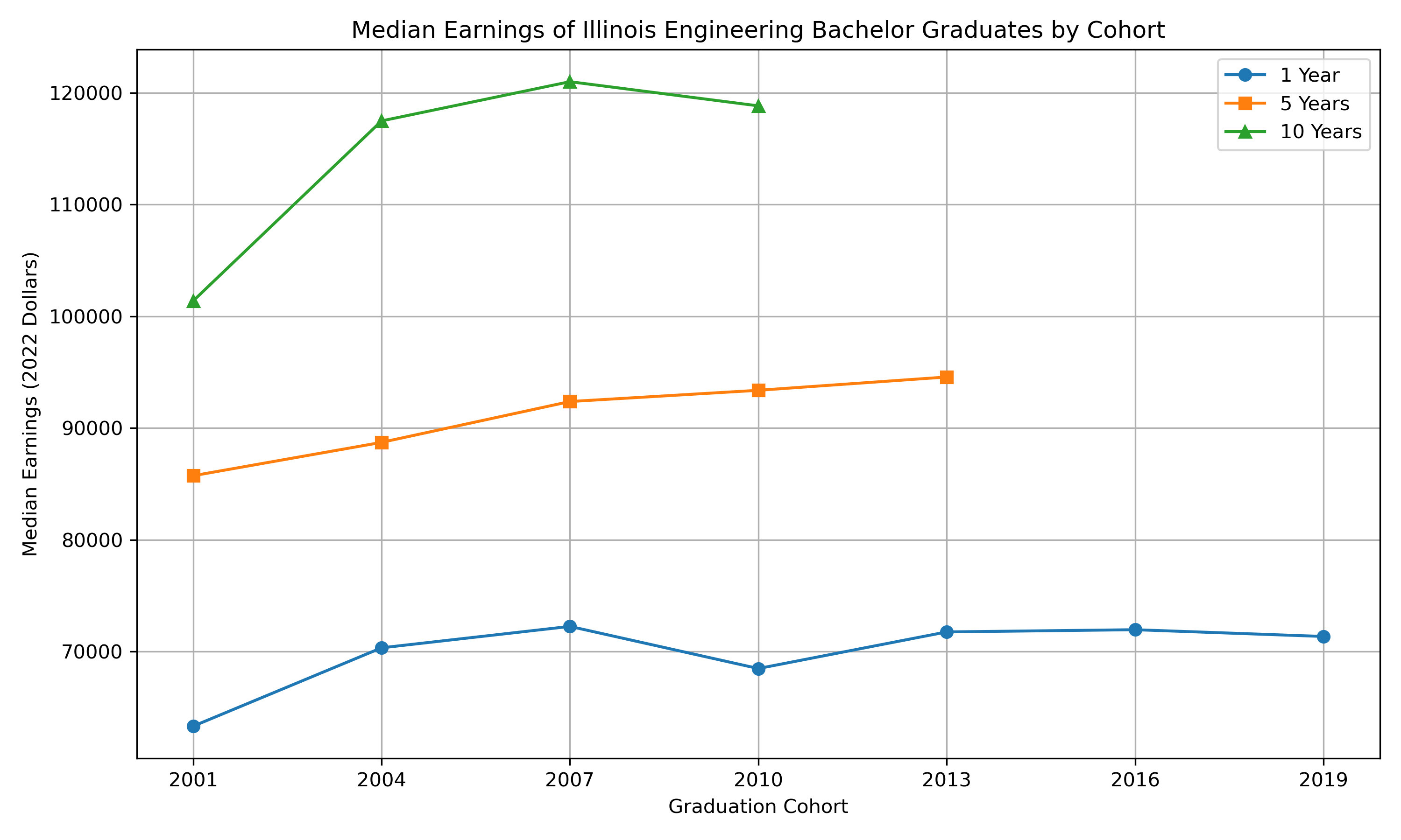
# Reshape data for plotting
df_long <- df %>%
  select(grad_cohort, y1_p50_earnings, y5_p50_earnings, y10_p50_earnings) %>%
  pivot_longer(
    cols = starts_with("y"),
    names_to = "years_after_grad",
    values_to = "earnings"
  )

# Clean label names for legend
df_long$years_after_grad <- recode(df_long$years_after_grad,
  y1_p50_earnings = "1 Year",
  y5_p50_earnings = "5 Years",
  y10_p50_earnings = "10 Years"
)

# Order for legend display
df_long$years_after_grad <- factor(df_long$years_after_grad,
  levels = c("1 Year", "5 Years", "10 Years")
)

# Plotting by cohort over time
ggplot(df_long, aes(x = grad_cohort, y = earnings, color = years_after_grad, group = years_after_grad)) +
  geom_line() +
  geom_point() +
  labs(
    title = "Median Earnings of Illinois Engineering Bachelor Graduates by Cohort",
    x = "Graduation Cohort",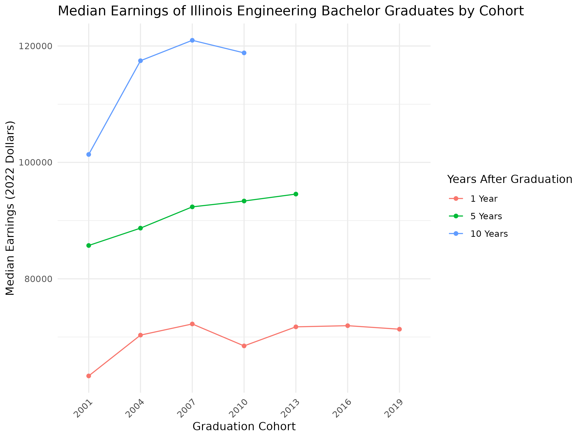
Case Study: How Many Engineering Graduates Stay in Illinois?
This case study examines the flows side of PSEO data, to help answer the question: “how many engineering bachelor’s graduates stay in state?” Instead of looking at all engineering graduates from Illinois, we will narrow it down to just the University of Illinois’ main campus, Urbana-Champaign. We want to know the number of graduates with a bachelor’s degree in engineering that are working in-state 1 year after graduation over time (i.e. by cohort). We can separate out this analysis by industry, looking at just the top 3 industries that graduates are working in.
The first step is to narrow the data down to the data we are interested in, which requires figuring out which institution code corresponds with the university. The code below loads in two schema files in addition to the data. The institution schema file contains all the institutions with their institution code (OPEID) and corresponding label. As we can see below, there are several labels associated with University of Illinois at Urbana-Champaign, but for our purposes, we can use the main code, “00177500”.
import pandas as pd

STATE = "il"
DATA_BASE_URL = "https://lehd.ces.census.gov/data/pseo/latest_release/"
SCHEMA_BASE_URL = "https://lehd.ces.census.gov/data/schema/latest/"

# Read in illinois flows CSV (gzipped)
il_flows = pd.read_csv(
    f"{DATA_BASE_URL}{STATE}/pseof_{STATE}.csv.gz",
    dtype={
        "institution": str,
        "degree_level": str,
        "cipcode": str,
        "cip_level": str,
        "grad_cohort": str,
        "industry": str,
    },
)

# Read in schema files - industry and institution
inst_labels = pd.read_csv(
    f"{SCHEMA_BASE_URL}label_institution.csv", dtype={"institution": str}
)
ind_labels = pd.read_csv(f"{SCHEMA_BASE_URL}label_industry.csv")

# Find institution label of University of Illinois
find_label = inst_labels[
    inst_labels["label"].str.contains(
        "University of Illinois Urbana-Champaign", na=False
    )
]

print(find_label[["institution", "label"]])
>> institution label >> 5922 00177500 University of Illinois Urbana-Champaign >> 5935 00177513 University of Illinois Urbana-Champaign - Nat'... >> 5938 00177516 University of Illinois Urbana-Champaign - Illi... >> 5939 00177517 University of Illinois Urbana-Champaign - Illi... >> 5940 00177518 University of Illinois Urbana-Champaign - Oakt...
library(readr)
library(dplyr)
library(stringr)

STATE <- "il"
DATA_BASE_URL <- "https://lehd.ces.census.gov/data/pseo/latest_release/"
SCHEMA_BASE_URL <- "https://lehd.ces.census.gov/data/schema/latest/"

# Read in illinois flows CSV (gzipped)
il_flows <- read_csv(
  paste0(DATA_BASE_URL, STATE, "/pseof_", STATE, ".csv.gz"),
  col_types = cols(
    institution = col_character(),
    degree_level = col_character(),
    cip_level = col_character(),
    cipcode = col_character(),
    grad_cohort = col_character(),
    industry = col_character(),
  )
)

# Read in schema files - industry and institution
inst_labels <- read_csv(
  paste0(SCHEMA_BASE_URL, "label_institution.csv"),
  col_types = cols(institution = col_character())
)
ind_labels <- read_csv(paste0(SCHEMA_BASE_URL, "label_industry.csv"))

# Find institution label of University of Illinois
find_label <- inst_labels %>%
  filter(str_detect(label, "University of Illinois Urbana-Champaign"))

print(select(find_label, institution, label))
>> # A tibble: 5 × 2 >> institution label >> <chr> <chr> >> 1 00177500 University of Illinois Urbana-Champaign >> 2 00177513 University of Illinois Urbana-Champaign - Nat'l Univ of Singapore >> 3 00177516 University of Illinois Urbana-Champaign - Illinois Center for Reh… >> 4 00177517 University of Illinois Urbana-Champaign - Illini Center and Chica… >> 5 00177518 University of Illinois Urbana-Champaign - Oakton Community College
Now that we know the institution code, we can limit the data to just those rows (as well as filtering for degree type, degree program, and geography). We want to visualize the share of graduates staying in state for the top three industries. To find the top three industries, we can use the “all cohorts” rows to determine across all cohorts which industries have the highest number of graduates working 1 year after graduation.
# Limit data to just relevant rows, bachelor's degree in engineering from university of illinois
il_flows = il_flows[il_flows["degree_level"] == "05"]
il_flows = il_flows[il_flows["cipcode"] == "14"]
il_flows = il_flows[il_flows["institution"] == "00177500"]

# The national geographic flow contains instate graduates as well as total graduates
il_flows = il_flows[il_flows["geo_level"] == "N"]

# Join industry labels to the data
il_flows = il_flows.merge(ind_labels, how="left", on="industry")

# Remove all industry row
il_flows = il_flows[il_flows["industry"] != "00"]

# Find top industries (use all cohort row)
all_cohorts = il_flows[il_flows["grad_cohort"] == "0000"]
top_industries = all_cohorts.sort_values("y1_grads_emp", ascending=False)[
    ["industry", "y1_grads_emp", "label"]
]

# View top industries
print(top_industries.iloc[0:3, :])
>> industry y1_grads_emp label >> 18 54 4273.0 Professional, Scientific, and Technical Services >> 11 31-33 4071.0 Manufacturing >> 15 51 867.0 Information
il_flows <- il_flows %>%
  filter(degree_level == "05") %>%
  filter(cipcode == "14") %>%
  filter(institution == "00177500")

# The national geographic flow contains instate graduates as well as total graduates
il_flows <- il_flows %>%
  filter(geo_level == "N")

# Join industry labels to the data
il_flows <- il_flows %>%
  left_join(ind_labels, by = "industry")

# Remove all industry row
il_flows <- il_flows %>%
  filter(industry != "00")

# Find top industries (use all cohort row)
all_cohorts <- il_flows %>%
  filter(grad_cohort == "0000")

top_industries <- all_cohorts %>%
  arrange(desc(y1_grads_emp)) %>%
  select(industry, y1_grads_emp, label)

# View top industries
print(head(top_industries, 3))
>> # A tibble: 3 × 3 >> industry y1_grads_emp label >> <chr> <dbl> <chr> >> 1 54 4273 Professional, Scientific, and Technical Services >> 2 31-33 4071 Manufacturing >> 3 51 867 Information
Now, we need to filter our data to just those rows in the top three industries. Then, we can create the “share of graduates in state” variable, and plot the data over the cohorts.
import matplotlib.pyplot as plt

# Limit to just the top three industries
top_three_inds = top_industries.iloc[0:3, 0]
il_flows = il_flows[il_flows["industry"].isin(top_three_inds)]

# Create share in-state variables
il_flows["share_instate"] = il_flows["y1_grads_emp_instate"] / il_flows["y1_grads_emp"]

# Remove all cohorts rows
il_flows = il_flows[il_flows["grad_cohort"] != "0000"]

# Ensure grad_cohort is sorted
il_flows = il_flows.sort_values("grad_cohort")

# Plot
plt.figure(figsize=(12, 6))

for label in il_flows["label"].unique():
    industry_data = il_flows[il_flows["label"] == label]
    # Sort by cohort to ensure lines are correct
    industry_data = industry_data.sort_values("grad_cohort")
    plt.plot(
        industry_data["grad_cohort"],
        industry_data["share_instate"],
        marker="o",
        label=label,
    )


plt.title("Share of Engineering Graduates from University of Illinois In-State")
plt.xlabel("Graduation Cohort")
plt.ylabel("Share of Graduates In-State 1-Year Post Graduation")
plt.legend()
plt.grid(True)
plt.tight_layout()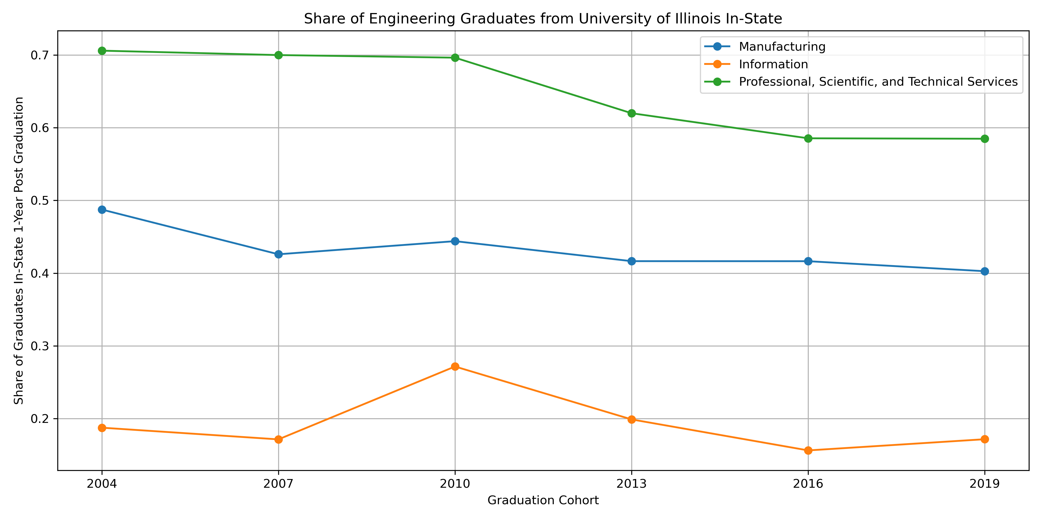
# Limit to just the top three industries
top_three_inds <- top_industries$industry[1:3]
il_flows <- il_flows %>%
  filter(industry %in% top_three_inds)

# Create share in-state variables
il_flows <- il_flows %>%
  mutate(share_instate = y1_grads_emp_instate / y1_grads_emp)

# Remove all cohort rows
il_flows <- il_flows %>%
  filter(grad_cohort != "0000")

# Ensure grad_cohort is sorted
il_flows <- il_flows %>%
  mutate(grad_cohort = as.integer(grad_cohort)) %>%
  arrange(grad_cohort)

# Plot
p <- ggplot(il_flows, aes(x = grad_cohort, y = share_instate, color = label, group = label)) +
  geom_line(size = 1) +
  geom_point() +
  labs(
    title = "Share of Engineering Graduates from University of Illinois In-State",
    x = "Graduation Cohort",
    y = "Share of Graduates In-State 1-Year Post Graduation",
    color = "Industry"
  ) +
  theme_minimal() +
  theme(legend.position = "right")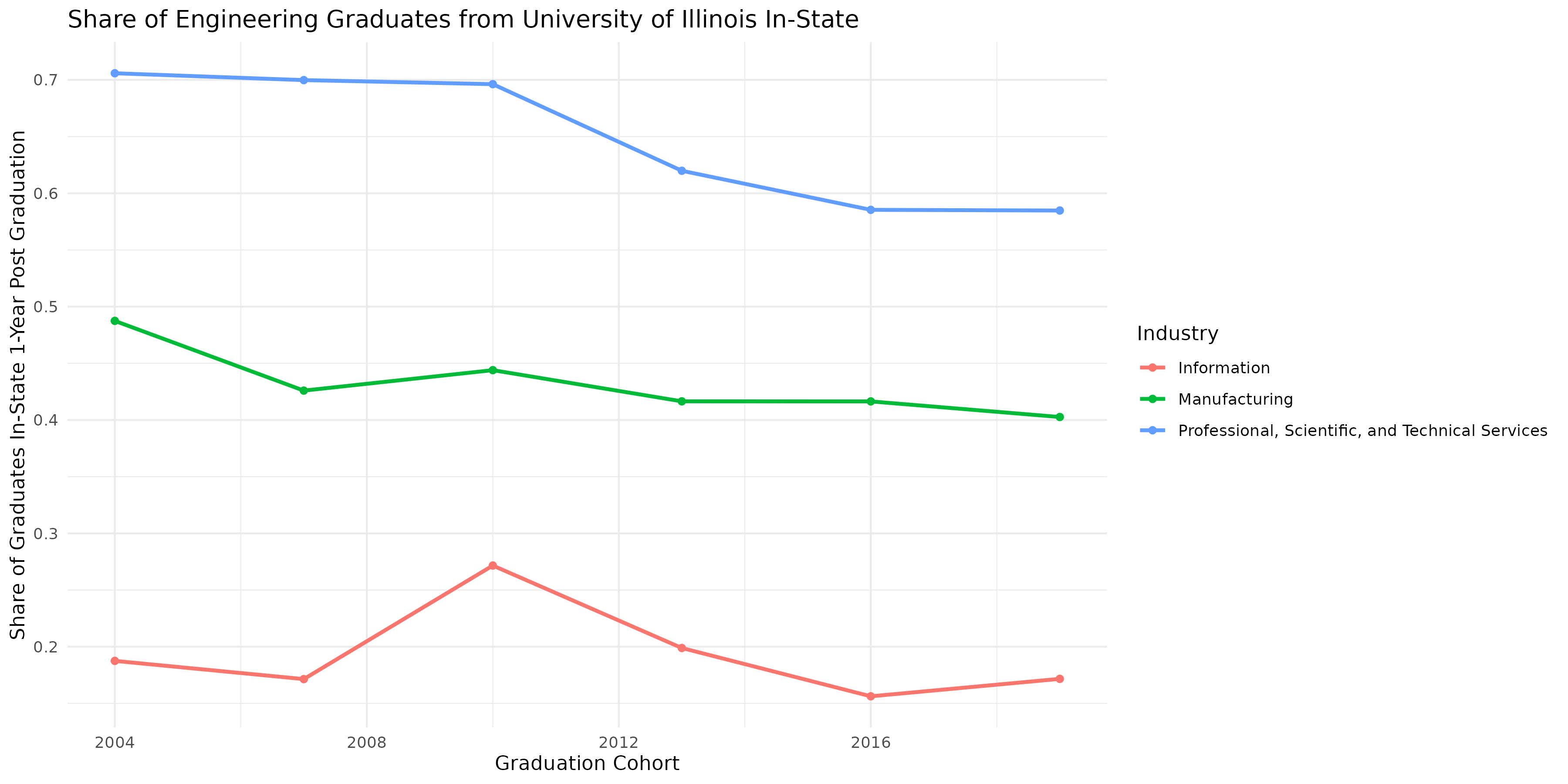
State Data Comparisons
Another data analysis that users may wish to do is comparing flows and/or earnings data across states (which is not easily accessible in PSEO Explorer). This is relatively simple to do, but does require either reading the entire PSEO files, or combining files from different states
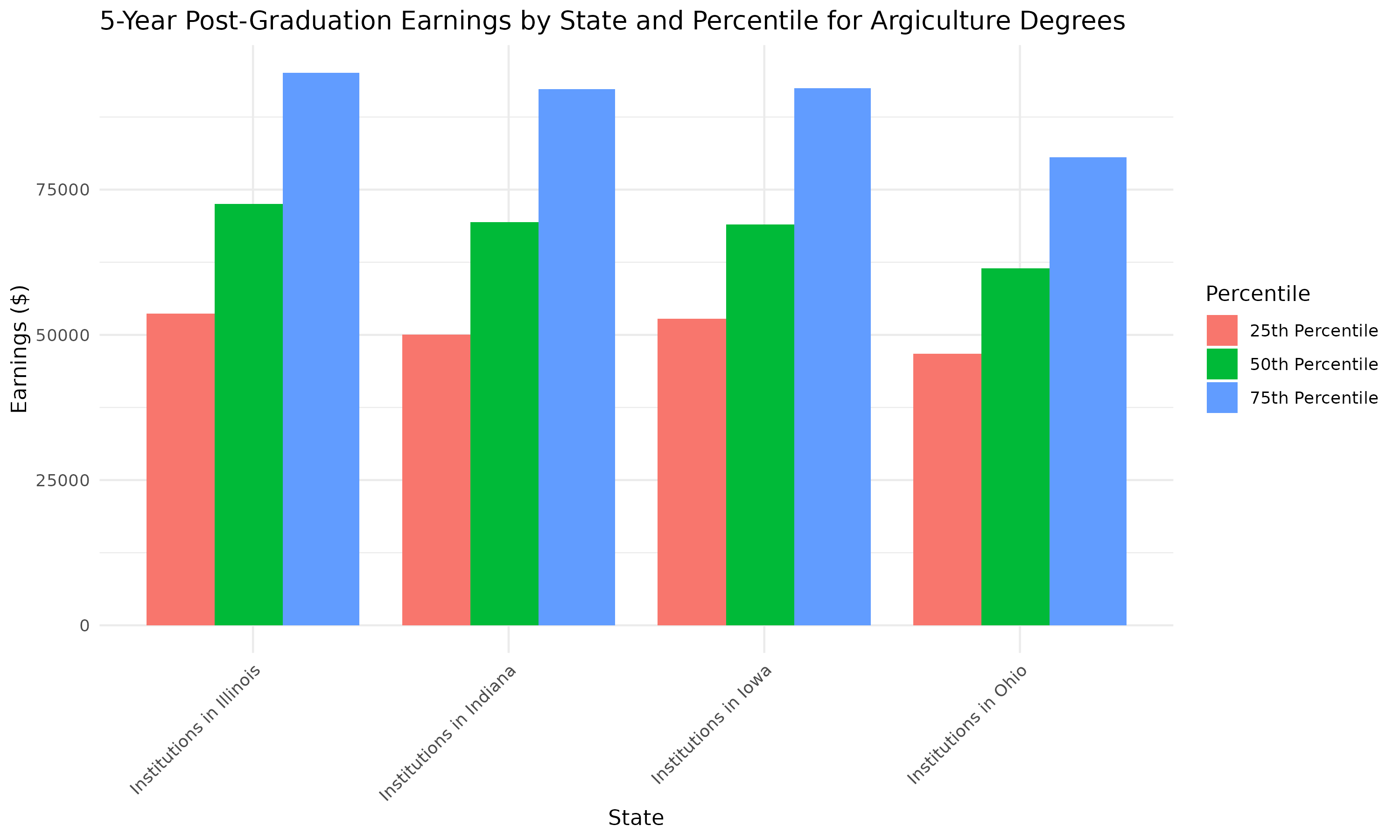
Case Study: Comparing Earnings in Agriculture Degrees in the Midwest
Here, we will be obtaining and plotting the earnings for agricultural degree at the state level for selected states in the Midwest. The first step here, is to decide which CIP code to use for our interest in “Agriculture”. There are 3 levels of CIP codes available in PSEO earnings data: the top level is the all CIPs (all together), the middle level is the 2-digit CIP Codes, and the most detailed is the 4-digit CIP Codes. The 4-digit CIP codes are only available on the earnings data, and are not available on the flows data. To see the full list of CIP codes associated with Agriculture, we filter the CIP labels on “Agr”. We can see there is the 2-digit CIP code “01”, that corresponds to “Agricultural/Animal/Plant/Veterinary Science and Related Fields.” This may be too broad for us here. We can also see there are several 4-digit CIP codes that fall under that CIP code, as well as one that falls under the general “Engineering” CIP code. For these purposes, let’s go with the code “01.01”, which is “Agricultural Business and Management”.
import pandas as pd
import matplotlib.pyplot as plt
import numpy as np

STATES = ["il", "in", "oh", "ia"]
DATA_BASE_URL = "https://lehd.ces.census.gov/data/pseo/latest_release/"
SCHEMA_BASE_URL = "https://lehd.ces.census.gov/data/schema/latest/"


# Read in data for each state and combine
all_data = []
for state in STATES:
    state_data = pd.read_csv(
        f"{DATA_BASE_URL}{state}/pseoe_{state}.csv.gz",
        dtype={
            "institution": str,
            "degree_level": str,
            "cip_level": str,
            "cipcode": str,
            "grad_cohort": str,
        },
    )
    # limit to only state
    state_data = state_data[state_data["inst_level"] == "S"]
    all_data.append(state_data)

midwest_earnings = pd.concat(all_data)

# Read in labels for cipcodes
cip_label = pd.read_csv(f"{SCHEMA_BASE_URL}label_cipcode.csv")

# Find cip codes that are in the data
cips_in_data = cip_label[
    cip_label["cipcode"].isin(midwest_earnings["cipcode"].unique())
]

# View labels
print(cips_in_data.loc[cips_in_data["label"].str.contains("Agr"), ["cipcode", "label"]])
>> cipcode label >> 1 01 Agricultural/Animal/Plant/Veterinary Science a... >> 2 01.00 Agriculture, General >> 4 01.01 Agricultural Business and Management >> 12 01.02 Agricultural Mechanization >> 18 01.03 Agricultural Production Operations >> 28 01.04 Agricultural and Food Products Processing >> 31 01.05 Agricultural and Domestic Animal Services >> 50 01.07 International Agriculture >> 52 01.08 Agricultural Public Services >> 86 01.13 Agriculture/Veterinary Preparatory Programs >> 113 01.99 Agricultural/Animal/Plant/Veterinary Science a... >> 515 14.03 Agricultural Engineering
library(dplyr)
library(readr)
library(tidyr)
library(ggplot2)

STATES <- c("il", "in", "oh", "ia")
DATA_BASE_URL <- "https://lehd.ces.census.gov/data/pseo/latest_release/"
SCHEMA_BASE_URL <- "https://lehd.ces.census.gov/data/schema/latest/"

# Read in data for each state and combine
all_data <- list()

for (state in STATES) {
  state_url <- paste0(DATA_BASE_URL, state, "/pseoe_", state, ".csv.gz")

  state_data <- read_csv(
    state_url,
    col_types = cols(
      institution = col_character(),
      degree_level = col_character(),
      cip_level = col_character(),
      cipcode = col_character(),
      grad_cohort = col_character()
    )
  )

  # limit to only state
  state_data <- state_data %>% filter(inst_level == "S")
  all_data[[state]] <- state_data
}

midwest_earnings <- bind_rows(all_data)

# Read in labels for cipcodes
cip_label <- read_csv(paste0(SCHEMA_BASE_URL, "label_cipcode.csv"))

# Find cip codes that are in the data
cips_in_data <- cip_label %>%
  filter(cipcode %in% unique(midwest_earnings$cipcode))

# View labels
print(
  cips_in_data %>%
    filter(grepl("Agr", label)) %>%
    select(cipcode, label)
)
>> # A tibble: 12 × 2 >> cipcode label >> <chr> <chr> >> 1 01 Agricultural/Animal/Plant/Veterinary Science and Related Fields >> 2 01.00 Agriculture, General >> 3 01.01 Agricultural Business and Management >> 4 01.02 Agricultural Mechanization >> 5 01.03 Agricultural Production Operations >> 6 01.04 Agricultural and Food Products Processing >> 7 01.05 Agricultural and Domestic Animal Services >> 8 01.07 International Agriculture >> 9 01.08 Agricultural Public Services >> 10 01.13 Agriculture/Veterinary Preparatory Programs >> 11 01.99 Agricultural/Animal/Plant/Veterinary Science and Related Fields, Oth… >> 12 14.03 Agricultural Engineering
Now we can limit the data to only the degree we’re interested in. We can also limit it to only Bachelor’s degrees, and we can select the data from all cohorts. We also join the data to the institution schema, which has the names of the states (otherwise we only have the FIPs code). Then we can create a grouped bar chart to show the 25th, 50th, and 75th percentile earnings at 5 years after graduation.
# Filter data to right degree level, cipcode, and all cohorts
midwest_earnings = midwest_earnings[midwest_earnings["degree_level"] == "05"]
midwest_earnings = midwest_earnings[midwest_earnings["cipcode"] == "01.01"]
midwest_earnings = midwest_earnings[midwest_earnings["grad_cohort"] == "0000"]

# Join data to institution schema for state labels
inst_labels = pd.read_csv(
    f"{SCHEMA_BASE_URL}label_institution.csv", dtype={"institution": str}
)
midwest_earnings = midwest_earnings.merge(inst_labels, how="left", on="institution")

# Melt to long format
df_long = midwest_earnings.melt(
    id_vars="label",
    value_vars=["y5_p25_earnings", "y5_p50_earnings", "y5_p75_earnings"],
    var_name="percentile",
    value_name="earnings",
)

# Clean percentile names for display
df_long["percentile"] = df_long["percentile"].str.extract(r"y5_(p\d+)_earnings")[0]

# Pivot to make plotting easier
pivot = df_long.pivot(index="label", columns="percentile", values="earnings")
percentiles = ["p25", "p50", "p75"]  # Ensure order

# Map short codes to nicer legend labels
percentile_labels = {
    "p25": "25th Percentile",
    "p50": "50th Percentile",
    "p75": "75th Percentile",
}

# Plotting
x = np.arange(len(pivot))  # number of states
width = 0.25

fig, ax = plt.subplots(figsize=(10, 6))


for i, p in enumerate(percentiles):
    ax.bar(x + i * width, pivot[p], width=width, label=percentile_labels[p])

# Customize axes
ax.set_xticks(x + width)
ax.set_xticklabels(pivot.index)
ax.set_ylabel("Earnings ($)")
ax.set_title(
    "5-Year Post-Graduation Earnings by State and Percentile for Argiculture Degrees"
)
ax.legend(title="Percentile")
ax.grid(True, axis="y")
plt.tight_layout()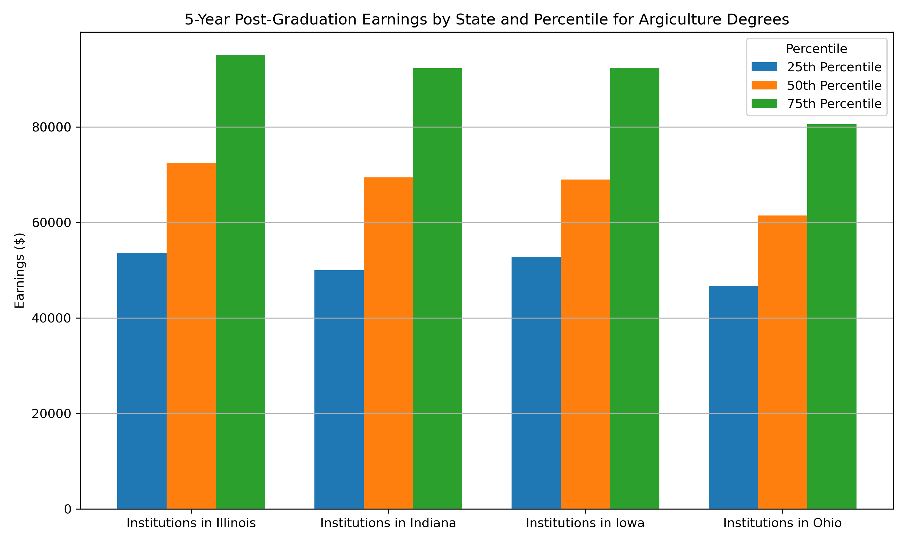
# Filter data to right degree level, cipcode, and all cohorts
midwest_earnings <- midwest_earnings %>%
  filter(degree_level == "05", cipcode == "01.01", grad_cohort == "0000")

# Join data to institution schema for state labels
inst_labels <- read_csv(
  paste0(SCHEMA_BASE_URL, "label_institution.csv"),
  col_types = cols(institution = col_character())
)

midwest_earnings <- midwest_earnings %>%
  left_join(inst_labels, by = "institution")

# Melt to long format
df_long <- midwest_earnings %>%
  pivot_longer(
    cols = c(y5_p25_earnings, y5_p50_earnings, y5_p75_earnings),
    names_to = "percentile",
    values_to = "earnings"
  )

# Clean percentile names for display
df_long <- df_long %>%
  mutate(percentile = gsub("y5_(p\\d+)_earnings", "\\1", percentile))

# Ensure ordering
df_long$percentile <- factor(df_long$percentile,
  levels = c("p25", "p50", "p75"),
  labels = c(
    "25th Percentile",
    "50th Percentile",
    "75th Percentile"
  )
)

# Plot
plot <- ggplot(df_long, aes(x = label, y = earnings, fill = percentile)) +
  geom_bar(stat = "identity", position = position_dodge(width = 0.8)) +
  labs(
    title = "5-Year Post-Graduation Earnings by State and Percentile for Argiculture Degrees",
    x = "State",
    y = "Earnings ($)",
    fill = "Percentile"
  ) +
  theme_minimal() +
  theme(axis.text.x = element_text(angle = 45, hjust = 1))