
2. A Full LODES Example
The previous section, LODES Code Building Blocks, focused on individual specific tasks that are useful for LODES data, including simple tasks, such as reading in data, as well as more complicated tasks, including merges, filters, and spatial analyses. Now, we will use these building blocks to answer a more complicated question. We will try to answer the following question: How many workers have a residence and a workplace within 0.5 miles of WMATA metro stations by year between 2016 and 2022? The Washington Metropolitan Area Transit Authority (WMATA) is the regional public transit agency that operates transportation services in the Washington, D.C. metropolitan area.
This task will be broken down into specific steps as follows:
Read in appropriate data files, both from LODES and for geographic WMATA data.
Find all Census blocks with centroids within 0.5 miles of metro stations.
Find all workers (by year) that have workplace and residence within 0.5 miles of metro stations.
2.1. Loading Appropriate Data Files
To be able to complete the above, we will need to read in multiple files. We will need geographic data to represent the location of WMATA stations, Origin-Destination (OD) LODES files to represent workers, and LODES geographic crosswalk files to find and filter the geographic location of Census Blocks. Each of these data files are detailed below:
WMATA Station Locations: Geographic data (shapefile) on WMATA metro station locations can be downloaded from this site.
LODES OD Files: The Origin-Destination files will provide data on worker residences and workplaces.
LODES Geographic Crosswalks: The crosswalks will provide the latitude and longitude of the census blocks for spatial merging.
2.1.1. Reading in WMATA Data
To read the WMATA data in, we will need to use a package that can handle spatial data. Note that this data includes some metro stations that were not open during all years in the analysis. This includes the Silver Line Phase 2 extension, which opened in late 2022, and the Potomac Yard infill station which opened in 2023. We should remove these stations from the dataset to ensure that the analysis is consistent.
import geopandas as gpd

# Read in WMATA data
metro_stations = gpd.read_file("data/wmata_metro_stations/")

# Remove metro stations that were not in service
stations_to_remove = [961, 732, 733, 734, 735, 736, 737]
metro_stations = metro_stations[~metro_stations["OBJECTID"].isin(stations_to_remove)]

# Convert to projection for contiguous USA
metro_stations = metro_stations.to_crs("ESRI:102003")

print(metro_stations.head())
>> NAME ... geometry >> 0 Branch Ave ... POINT (1630721.601 312999.777) >> 1 Braddock Road ... POINT (1619008.366 309217.01) >> 2 King St-Old Town ... POINT (1618573.732 308265.011) >> 3 Eisenhower Ave ... POINT (1617861.758 307416.8) >> 4 Huntington ... POINT (1617640.802 306627.861) >> >> [5 rows x 15 columns]
library(sf)
library(dplyr)

# Read in WMATA data (assumes GeoPackage, Shapefile, or similar)
metro_stations <- st_read("data/wmata_metro_stations/", quiet = TRUE)

# Remove metro stations that were not in service
stations_to_remove <- c(961, 732, 733, 734, 735, 736, 737)
metro_stations <- metro_stations %>%
  filter(!OBJECTID %in% stations_to_remove)

# Convert to projection for contiguous USA
metro_stations <- st_transform(metro_stations, crs = "ESRI:102003")

# Print the first few rows
print(head(metro_stations))
>> Simple feature collection with 6 features and 14 fields >> Geometry type: POINT >> Dimension: XY >> Bounding box: xmin: 1617641 ymin: 306627.9 xmax: 1630722 ymax: 315574.5 >> Projected CRS: USA_Contiguous_Albers_Equal_Area_Conic >> NAME ADDRESS LINE >> 1 Branch Ave 4704 OLD SOPER ROAD, SUITLAND, MD green >> 2 Braddock Road 700 N. WEST ST., ALEXANDRIA, VA blue, yellow >> 3 King St-Old Town 1900 KING STREET, ALEXANDRIA, VA blue, yellow >> 4 Eisenhower Ave 2400 EISENHOWER AVENUE, ALEXANDRIA, VA yellow >> 5 Huntington 2701 HUNTINGTON AVENUE, ALEXANDRIA, VA yellow >> 6 Anacostia 1101 HOWARD ROAD SE, WASHINGTON, DC green >> TRAININFO_ >> 1 https://www.wmata.com/js/nexttrain/nexttrain.html#F11|Branch Ave >> 2 https://www.wmata.com/js/nexttrain/nexttrain.html#C12|Braddock Road >> 3 https://www.wmata.com/js/nexttrain/nexttrain.html#C13|King St-Old Town >> 4 https://www.wmata.com/js/nexttrain/nexttrain.html#C14|Eisenhower Avenue >> 5 https://www.wmata.com/js/nexttrain/nexttrain.html#C15|Huntington >> 6 https://www.wmata.com/js/nexttrain/nexttrain.html#F06|Anacostia >> WEB_URL >> 1 https://www.wmata.com/rider-guide/stations/branch-ave.cfm >> 2 https://www.wmata.com/rider-guide/stations/braddock-rd.cfm >> 3 https://www.wmata.com/rider-guide/stations/king-street.cfm >> 4 https://www.wmata.com/rider-guide/stations/eisenhower-ave.cfm >> 5 https://www.wmata.com/rider-guide/stations/huntington.cfm >> 6 https://www.wmata.com/rider-guide/stations/anacostia.cfm >> GIS_ID MAR_ID GLOBALID OBJECTID >> 1 MetroStnFullPt_35 NA {92A8B776-C7DD-4E1A-A9BF-83DBBFE3320F} 641 >> 2 MetroStnFullPt_36 NA {29FC24FF-2132-4F11-9D55-00ED0AD62B0E} 642 >> 3 MetroStnFullPt_37 NA {AC34C280-68C2-473F-88C6-7178859F27F1} 643 >> 4 MetroStnFullPt_38 NA {C137D724-61A0-4191-A166-14CADEF67A07} 644 >> 5 MetroStnFullPt_39 NA {68ACB463-D755-47C0-8907-AF039EDA5A8E} 645 >> 6 MetroStnFullPt_40 294866 {9F18B9CF-3BD8-4F44-8E93-945E4094B4BF} 646 >> CREATOR CREATED EDITOR EDITED SE_ANNO_CA geometry >> 1 JLAY 2022-11-30 JLAY 2022-11-30 <NA> POINT (1630722 312999.8) >> 2 JLAY 2022-11-30 JLAY 2022-11-30 <NA> POINT (1619008 309217) >> 3 JLAY 2022-11-30 JLAY 2022-11-30 <NA> POINT (1618574 308265) >> 4 JLAY 2022-11-30 JLAY 2022-11-30 <NA> POINT (1617862 307416.8) >> 5 JLAY 2022-11-30 JLAY 2022-11-30 <NA> POINT (1617641 306627.9) >> 6 JLAY 2022-11-30 JLAY 2022-11-30 <NA> POINT (1622836 315574.5)
2.1.2. Reading in LODES Data
We need LODES files for DC, Maryland, and Virginia (the three states that have WMATA metro stations) and across the years specified in the problem. For this problem, we have chosen the job type “JT01”, which corresponds to the “Primary Jobs.” This was chosen here because we are interested in individuals, and not jobs (of which an individual can have more than one). We will require both “main” and “auxiliary” files, since we need workers with workplaces in the same state as their residence well as workers that have a residence in other states.
In addition to the OD data, we will need the geographic crosswalks for each of the states. We can use the functions we wrote in Loading Data to load in all the necessary LODES data.
import pandas as pd

# Read in OD data
all_od = []
states = ["dc", "va", "md"]

# Years between 2016 (inclusive) and 2023 (exclusive)
year_range = list(range(2016, 2023))
for state in states:
    for year in year_range:
        main = read_lodes_data(
            data_type="od",
            state=state,
            segment=None,
            job_type="JT01",
            year=year,
            main=True,
        )
        main["year"] = year
        all_od.append(main)
        aux = read_lodes_data(
            data_type="od",
            state=state,
            segment=None,
            job_type="JT01",
            year=year,
            main=False,
        )
        aux["year"] = year
        all_od.append(aux)

# Concatenate all OD files
all_od = pd.concat(all_od)

# Read in crosswalk files
all_crosswalks = []
for state in states:
    all_crosswalks.append(read_crosswalk(state=state, cols=["blklatdd", "blklondd"]))

# Concatenate all crosswalks
all_crosswalks = pd.concat(all_crosswalks)

print(all_od.head())
>> w_geocode h_geocode S000 SA01 ... SI02 SI03 createdate year >> 0 110010001011000 110010003001003 1 1 ... 0 1 20230321 2016 >> 1 110010001011000 110010039022000 1 0 ... 0 1 20230321 2016 >> 2 110010001011000 110010043002000 1 0 ... 0 1 20230321 2016 >> 3 110010001011000 110010089032004 1 0 ... 0 1 20230321 2016 >> 4 110010001011000 110010106023005 1 0 ... 0 1 20230321 2016 >> >> [5 rows x 14 columns]
library(dplyr)
library(purrr)

# Read in OD data
states <- c("dc", "va", "md")
year_range <- 2016:2022

all_od <- map_dfr(states, function(state) {
  map_dfr(year_range, function(year) {
    main_data <- read_lodes_data(
      data_type = "od",
      state = state,
      segment = NULL,
      job_type = "JT01",
      year = year,
      main = TRUE
    ) %>%
      mutate(year = year)

    aux_data <- read_lodes_data(
      data_type = "od",
      state = state,
      segment = NULL,
      job_type = "JT01",
      year = year,
      main = FALSE
    ) %>%
      mutate(year = year)

    bind_rows(main_data, aux_data)
  })
})

# Read in crosswalk files
all_crosswalks <- map_dfr(states, function(state) {
  read_crosswalk(state = state, cols = c("blklatdd", "blklondd"))
})

print(head(all_od))
>> # A tibble: 6 × 14 >> w_geocode h_geocode S000 SA01 SA02 SA03 SE01 SE02 SE03 SI01 SI02 >> <chr> <chr> <dbl> <dbl> <dbl> <dbl> <dbl> <dbl> <dbl> <dbl> <dbl> >> 1 1100100010110… 11001000… 1 1 0 0 0 1 0 0 0 >> 2 1100100010110… 11001003… 1 0 1 0 0 0 1 0 0 >> 3 1100100010110… 11001004… 1 0 1 0 0 0 1 0 0 >> 4 1100100010110… 11001008… 1 0 1 0 0 0 1 0 0 >> 5 1100100010110… 11001010… 1 0 1 0 0 0 1 0 0 >> 6 1100100010110… 11001000… 1 0 0 1 0 0 1 0 0 >> # ℹ 3 more variables: SI03 <dbl>, createdate <dbl>, year <int>
2.2. Finding Census Blocks Near Metro Stations
To find the census blocks within 0.5 miles of the metro stations, we must add a buffer to our metro stations. This code adds the buffer in meters (since the projection is in meters) and plots the resulting data.
import matplotlib.pyplot as plt

# Buffer metro stations by 805 meters (approximately 0.5 miles)
metro_stations["geometry"] = metro_stations.geometry.buffer(805)

# Create plot and plot stations
fig, ax = plt.subplots()
metro_stations.plot(ax=ax, color="lightblue", edgecolor="black")

# Add title
ax.set_title("Buffered WMATA Metro Stations", fontsize=14)
ax.grid(True, linestyle="--", linewidth=0.5, alpha=0.7)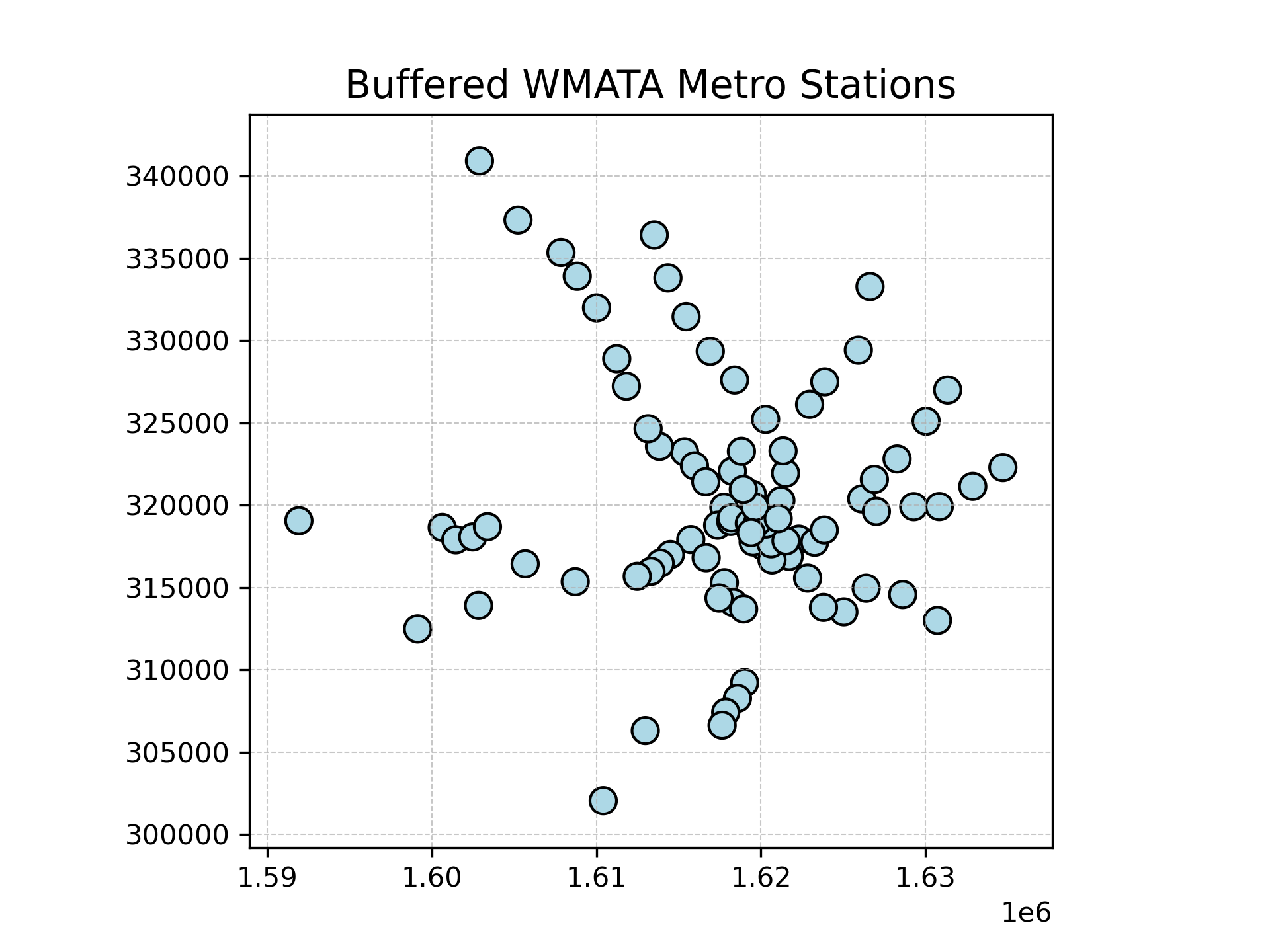
library(ggplot2)
print(metro_stations)

# Buffer stations by 805 meters (approximately 0.5 miles)
# Match the resolution (nQuadSegs) to that used by Python.
metro_stations$geometry <- st_buffer(metro_stations$geometry, dist = 805, nQuadSegs = 16)

# Plot stations
ggplot(data = metro_stations) +
  geom_sf(fill = "lightblue", color = "black") +
  ggtitle("Buffered WMATA Metro Stations") +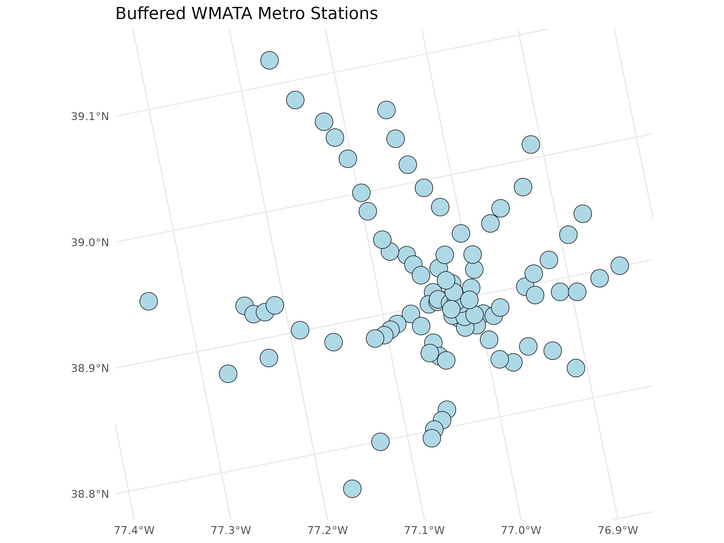
Next, we need to find the Census blocks which have internal points within the buffered metro stations. To do this, we can use a spatial join between our metro stations and the crosswalks. First we need to convert the projection of the crosswalk file to the same projection as the metro stations. Then we can use a spatial join to find all the blocks that have internal points within the buffer. We do this by finding the blocks that have internal points that “intersect” with the buffered WMATA polygons.
# Convert crosswalk to geographic dataframe
all_crosswalks = gpd.GeoDataFrame(
    all_crosswalks,
    geometry=gpd.points_from_xy(all_crosswalks["blklondd"], all_crosswalks["blklatdd"]),
    crs="EPSG:4326",
)

# Convert to projection for contiguous USA
all_crosswalks = all_crosswalks.to_crs("ESRI:102003")

# Spatial join using 'intersects'
blocks_within_buffers = gpd.sjoin(
    all_crosswalks, metro_stations, predicate="intersects"
)

print(blocks_within_buffers.head())
>> tabblk2020 blklatdd blklondd ... EDITOR EDITED SE_ANNO_CA >> 2 110010001011002 38.9090878 -77.0508394 ... JLAY 2022-11-30 None >> 3 110010001011003 38.9094979 -77.0514369 ... JLAY 2022-11-30 None >> 61 110010001023020 38.9051080 -77.0571913 ... JLAY 2022-11-30 None >> 62 110010001023021 38.9043208 -77.0562779 ... JLAY 2022-11-30 None >> 63 110010001023022 38.9049298 -77.0558271 ... JLAY 2022-11-30 None >> >> [5 rows x 19 columns]
# Convert crosswalk to geographic dataframe
all_crosswalks <- st_as_sf(all_crosswalks, coords = c("blklondd", "blklatdd"), crs = 4326)

# Convert to projection for contiguous USA
all_crosswalks <- st_transform(all_crosswalks, crs = 102003)

# Spatial join using 'intersects'
blocks_within_buffers <- st_join(all_crosswalks, metro_stations, join = st_within, left = FALSE)

print(head(blocks_within_buffers))
>> Simple feature collection with 6 features and 15 fields >> Geometry type: POINT >> Dimension: XY >> Bounding box: xmin: 1616673 ymin: 318847.8 xmax: 1617139 ymax: 319730.2 >> Projected CRS: USA_Contiguous_Albers_Equal_Area_Conic >> # A tibble: 6 × 16 >> tabblk2020 geometry NAME ADDRESS LINE TRAININFO_ WEB_URL >> <chr> <POINT [m]> <chr> <chr> <chr> <chr> <chr> >> 1 110010001011… (1617139 319695.3) Dupont Circ… 1525 2… red https://w… https:… >> 2 110010001011… (1617080 319730.2) Dupont Circ… 1525 2… red https://w… https:… >> 3 110010001023… (1616693 319150) Foggy Botto… 890 23… blue… https://w… https:… >> 4 110010001023… (1616787 319079) Foggy Botto… 890 23… blue… https://w… https:… >> 5 110010001023… (1616812 319153.6) Foggy Botto… 890 23… blue… https://w… https:… >> 6 110010001023… (1616673 318847.8) Foggy Botto… 890 23… blue… https://w… https:… >> # ℹ 9 more variables: GIS_ID <chr>, MAR_ID <int>, GLOBALID <chr>, >> # OBJECTID <int>, CREATOR <chr>, CREATED <date>, EDITOR <chr>, EDITED <date>, >> # SE_ANNO_CA <chr>
2.3. Find Workers with Residence and Workplace Near Metro
Now that we have a list of Census blocks within the metro station buffers, we can limit our full data file to just those rows that represent workers with workplaces and residences within 0.5 miles of a metro station. Then, finally, we can group by year and display the result.
# Get list of blocks within the buffer
include_blocks = blocks_within_buffers["tabblk2020"].to_list()

# Filter for rows in which home and work are in buffered list
limited_od = all_od[
    (all_od["h_geocode"].isin(include_blocks))
    & (all_od["w_geocode"]).isin(include_blocks)
]

# Group and sum total jobs by year
jobs_by_year = limited_od[["S000", "year"]].groupby("year").sum().reset_index()

print(jobs_by_year)
>> year S000 >> 0 2016 163304 >> 1 2017 160919 >> 2 2018 164239 >> 3 2019 164884 >> 4 2020 165197 >> 5 2021 152995 >> 6 2022 159406
# Get list of blocks within the buffer
include_blocks <- blocks_within_buffers$tabblk2020

# Filter for rows where home and work geocodes are in the buffer
limited_od <- all_od %>%
  filter(h_geocode %in% include_blocks, w_geocode %in% include_blocks)

# Group and sum total jobs by year
jobs_by_year <- limited_od %>%
  group_by(year) %>%
  summarise(S000 = sum(S000, na.rm = TRUE), .groups = "drop")

print(jobs_by_year)
>> # A tibble: 7 × 2 >> year S000 >> <int> <dbl> >> 1 2016 163304 >> 2 2017 160919 >> 3 2018 164239 >> 4 2019 164884 >> 5 2020 165197 >> 6 2021 152995 >> 7 2022 159406